Fourier Transform¶

Background¶

Definition and basic properties¶

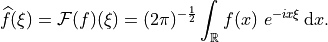
The Fourier Transform (FT) of a function $f$ belonging to the Lebesgue Space $L^1(\mathbb{R}, \mathbb{C})$ is defined as

(1)¶ $\widehat{f}(\xi) = \mathcal{F}(f)(\xi) = (2\pi)^{-\frac{1}{2}} \int_{\mathbb{R}} f(x)\ e^{-i x \xi} \, \mathrm{d}x.$

(Note that this definition differs from the one in the linked article by the placement of the factor $2\pi$ .) By unique continuation, the bounded FT operator can be extended to $L^p(\mathbb{R}, \mathbb{C})$ for $p \in [1, 2]$ , yielding a mapping

$\mathcal{F}: L^p(\mathbb{R}, \mathbb{C}) \longrightarrow L^q(\mathbb{R}, \mathbb{C}), \quad q = \frac{p}{p-1},$

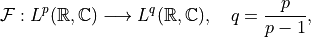
where $q$ is the conjugate exponent of $p$ (for $p=1$ one sets $q=\infty$ ). Finite exponents larger than 2 also allow the extension of the operator but require the notion of Distributions to characterize its range. See [SW1971] for further details.

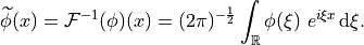
The inverse of $\mathcal{F}$ on its range is given by the formula

(2)¶ $\widetilde{\phi}(x) = \mathcal{F}^{-1}(\phi)(x) = (2\pi)^{-\frac{1}{2}} \int_{\mathbb{R}} \phi(\xi)\ e^{i \xi x}\, \mathrm{d}\xi.$

For $p = 2$ , the conjugate exponent is $q = 2$ , and the FT is a unitary operator on $L^2(\mathbb{R})$ according to Parseval’s Identity

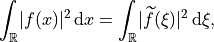
$\int_{\mathbb{R}} \lvert f(x)\rvert^2\, \mathrm{d}x = \int_{\mathbb{R}} \lvert \widetilde{f}(\xi) \rvert^2\, \mathrm{d}\xi,$

which implies that its adjoint is its inverse, $\mathcal{F}^* = \mathcal{F}^{-1}$ .

Further Properties¶

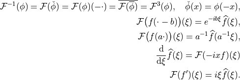
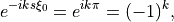
(3)¶ $\mathcal{F}^{-1}(\phi) = \mathcal{F}(\check\phi) = \mathcal{F}(\phi)(-\cdot) = \overline{\mathcal{F}(\overline{\phi})} = \mathcal{F}^3(\phi), \quad \check\phi(x) = \phi(-x), \mathcal{F}\big(f(\cdot - b)\big)(\xi) = e^{-i b \xi} \widehat{f}(\xi), \mathcal{F}\big(f(a \cdot)\big)(\xi) = a^{-1} \widehat{f}(a^{-1}\xi), \frac{\mathrm{d}}{\mathrm{d} \xi} \widehat{f}(\xi) = \mathcal{F}(-i x f)(\xi) \mathcal{F}(f')(\xi) = i \xi \widehat{f}(\xi).$

The first identity implies in particular that for real-valued 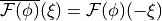$f$ , it is $\overline{\mathcal{F}(\phi)}(\xi) = \mathcal{F}(\phi)(-\xi)$ , i.e. the FT is completely known already from the its values in a half-space only. This property is later exploited to reduce storage.

In $d$ dimensions, the FT is defined as

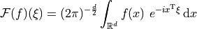
$\mathcal{F}(f)(\xi) = (2\pi)^{-\frac{d}{2}} \int_{\mathbb{R}^d} f(x)\ e^{-i x^{\mathrm{T}}\xi} \, \mathrm{d}x$

with the usual inner product 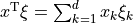$x^{\mathrm{T}}\xi = \sum_{k=1}^d x_k \xi_k$ in $\mathbb{R}^d$ . The identities (3) also hold in this case with obvious modifications.

Discretized Fourier Transform¶

General case¶

The approach taken in ODL for the discretization of the FT follows immediately from the way Discretizations are defined, but the original inspiration for it came from the book [Pre+2007], Section 13.9 “Computing Fourier Integrals Using the FFT”.

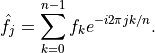
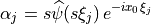
Discretization of the Fourier transform operator means evaluating the Fourier integral (1) on a discretized function

(4)¶ $f(x) = \sum_{k=0}^{n-1} f_k \phi_k(x)$

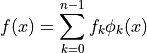
with coefficients 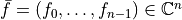$\bar f = (f_0, \dots, f_{n-1}) \in \mathbb{C}^n$ and functions $\phi_0, \dots, \phi_{n-1}$ . This approach follows from the way , but can be We consider in particular functions generated from a single kernel $\phi$ via

$\phi_k(x) = \phi\left( \frac{x - x_k}{s_k} \right),$

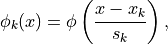
where $x_0 < \dots < x_{n-1}$ are sampling points and $s_k > 0$ scaling factors. Using the shift and scaling properties in (3) yields

(5)¶ $\widehat{f}(\xi) = \sum_{k=0}^{n-1} f_k \widehat{\phi_k}(\xi) = \sum_{k=0}^{n-1} f_k\, s_k \widehat{\phi}(s_k\xi) e^{-i x_k \xi}.$

There exist methods for the fast approximation of such sums for a general choice of frequency samples $\xi_m$ , e.g. NFFT.

Regular grids¶

For regular grids

(6)¶ $x_k = x_0 + ks, \quad \xi_j = \xi_0 + j\sigma,$

the evaluation of the integral can be written in the form which uses trigonometric sums as computed in FFTW or in Numpy:

(7)¶ $\hat f_j = \sum_{k=0}^{n-1} f_k e^{-i 2\pi jk/n}.$

Hence, the Fourier integral evaluation can be built around established libraries with simple pre- and post-processing steps.

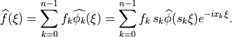
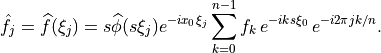
With regular grids, the discretized integral (5) evaluated at $\xi = \xi_j$ , can be expanded to

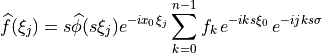
$\widehat{f}(\xi_j) = s \widehat{\phi}(s\xi_j) e^{-i x_0\xi_j} \sum_{k=0}^{n-1} f_k\, e^{-i k s \xi_0}\, e^{-i jk s\sigma}$

To reach the form (7), the factor depending on both indices $j$ and $k$ must agree with the corresponding factor in the FFT sum. This is achieved by setting

(8)¶ $\sigma = \frac{2\pi}{ns},$

finally yielding the representation

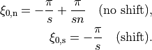
(9)¶ $\hat f_j = \widehat{f}(\xi_j) = s \widehat{\phi}(s\xi_j) e^{-i x_0\xi_j} \sum_{k=0}^{n-1} f_k\, e^{-i k s \xi_0}\, e^{-i 2\pi jk/n}.$

Choice of $\xi_0$ ¶

There is a certain degree of freedom in the choice of the most negative frequency $\xi_0$ . Usually one wants to center the Fourier space grid around zero since most information is typically concentrated there. Point-symmetric grids are the standard choice, however sometimes one explicitly wants to include (for even $n$ ) or exclude (for odd $n$ ) the zero frequency from the grid, which is achieved by shifting the frequency $xi_0$ by $-\sigma/2$ . This results in two possible choices

$\xi_{0, \mathrm{n}} = -\frac{\pi}{s} + \frac{\pi}{sn} \quad \text{(no shift)}, \xi_{0, \mathrm{s}} = -\frac{\pi}{s} \quad \text{(shift)}.$

For the shifted frequency, the pre-processing factor in the sum in (9) can be simplified to

$e^{-i k s \xi_0} = e^{i k \pi} = (-1)^k,$

which is favorable for real-valued input $\bar f$ since this first operation preserves this property. For half-complex transforms, shifting is required.

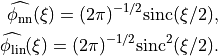
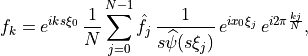
The factor $\widehat{\phi}(s\xi_j)$ ¶

In (9), the FT of the kernel $\phi$ appears as post-processing factor. We give the explicit formulas for the two standard discretizations currently used in ODL, which are nearest neighbor interpolation

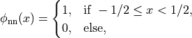
$\phi_{\mathrm{nn}}(x) = \begin{cases} 1, & \text{if } -1/2 \leq x < 1/2, \\ 0, & \text{else,} \end{cases}$

and linear interpolation

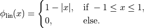
$\phi_{\mathrm{lin}}(x) = \begin{cases} 1 - \lvert x \rvert, & \text{if } -1 \leq x \leq 1, \\ 0, & \text{else.} \end{cases}$

Their Fourier transforms are given by

$\widehat{\phi_{\mathrm{nn}}}(\xi) = (2\pi)^{-1/2} \mathrm{sinc}(\xi/2), \widehat{\phi_{\mathrm{lin}}}(\xi) = (2\pi)^{-1/2} \mathrm{sinc}^2(\xi/2).$

Since their arguments 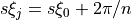$s\xi_j = s\xi_0 + 2\pi/n$ lie between $-\pi$ and $\pi$ , these functions introduce only a slight taper towards higher frequencies given the fact that the first zeros lie at $\pm 2\pi$ .

Inverse transform¶

According to (2), the inverse of the continuous Fourier transform is given by the same formula as the forward transform (1), except for a switched sign in the complex exponential. Hence, this operator can rather be viewed as a variation of the forward FT, and it is implemented via a sign parameter in FourierTransform.

The inverse of the discretized formula (9) is instead gained directly using the identity

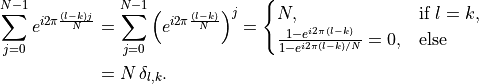
(10)¶ $\sum_{j=0}^{N-1} e^{i 2\pi \frac{(l-k)j}{N}} &= \sum_{j=0}^{N-1} \Big( e^{i 2\pi \frac{(l-k)}{N}} \Big)^j = \begin{cases} N, & \text{if } l = k, \\ \frac{1 - e^{i 2\pi (l-k)}}{1 - e^{i 2\pi (l-k)/N}} = 0, & \text{else} \end{cases}\\ &= N\, \delta_{l, k}.$

By dividing (9) with the factor

$\alpha_j = s\widehat{\psi}(s\xi_j)\, e^{- i x_0 \xi_j}$

before the sum, multiplying with the exponential factor $e^{i 2\pi \frac{lj}{N}}$ and summing over $j$ , the coefficients $f_k$ can be recovered:

$\sum_{j=0}^{N-1} \hat f_j\, \frac{1}{\alpha_j}\, e^{i 2\pi \frac{lj}{N}} &= \sum_{j=0}^{N-1} \sum_{k=0}^{N-1} \bar f_k\, e^{- i 2\pi \frac{jk}{N}} e^{i 2\pi \frac{lj}{N}} &= \sum_{k=0}^{N-1} \bar f_k\, N \delta_{l,k} &= N\, \bar f_l.$

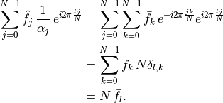
Hence, the inversion formula for the discretized FT reads as

(11)¶ $f_k = e^{i k s\xi_0}\, \frac{1}{N} \sum_{j=0}^{N-1} \hat f_j \, \frac{1}{s\widehat{\psi}(s\xi_j)}\, e^{i x_0\xi_j}\, e^{i 2\pi \frac{kj}{N}},$

which can be calculated in the same manner as the forward FT, basically by switching the roles of pre- and post-processing steps and flipping the sign in the complex exponentials.

Adjoint operator¶

If the FT is defined between the complex Hilbert spaces $L^2(\mathbb{R}, \mathbb{C})$ , one can easily show that the operator is unitary, and therefore its adjoint is equal to the inverse.

However, if the domain is a real space, $L^2(\mathbb{R}, \mathbb{C})$ , one cannot even speak of a linear operator since the property

$\mathcal{F}(\alpha f) = \alpha \mathcal{F}(f)$

cannot be tested for all $\alpha \in \mathbb{C}$ as required by the right-hand side, since on the left-hand side, $\alpha f$ needs to be real. This issue can be remedied by identifying the real and imaginary parts in the range with components of a product space element:

$\widetilde{\mathcal{F}}: L^2(\mathbb{R}, \mathbb{R}) \longrightarrow \big[L^2(\mathbb{R}, \mathbb{R})\big]^2, \widetilde{\mathcal{F}}(f) = \big(\Re \big(\mathcal{F}(f)\big), \Im \big(\mathcal{F}(f)\big)\big) = \big( \mathcal{F}_{\mathrm{c}}(f), -\mathcal{F}_{\mathrm{s}}(f) \big),$

where $\mathcal{F}_{\mathrm{c}}$ and $\mathcal{F}_{\mathrm{s}}$ are the sine and cosine transforms, respectively. Those two operators are self-adjoint between real Hilbert spaces, and thus the adjoint of the above defined transform is given by

$\widetilde{\mathcal{F}}^*: \big[L^2(\mathbb{R}, \mathbb{R})\big]^2 \longrightarrow L^2(\mathbb{R}, \mathbb{R}) \widetilde{\mathcal{F}}^*(g_1, g_2) = \mathcal{F}_{\mathrm{c}}(g_1) - \mathcal{F}_{\mathrm{s}}(g_2).$

If we compare this result to the “naive” approach of taking the real part of the inverse of the complex inverse transform, we get

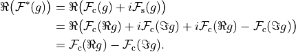
$\begin{align*} \Re\big( \mathcal{F}^*(g) \big) &= \Re\big( \mathcal{F}_{\mathrm{c}}(g) + i \mathcal{F}_{\mathrm{s}}(g) \big)\\ &= \Re\big( \mathcal{F}_{\mathrm{c}}(\Re g) + i \mathcal{F}_{\mathrm{c}}(\Im g) + i \mathcal{F}_{\mathrm{c}}(\Re g) - \mathcal{F}_{\mathrm{c}}(\Im g) \big)\\ &= \mathcal{F}_{\mathrm{c}}(\Re g) - \mathcal{F}_{\mathrm{c}}(\Im g). \end{align*}$

Hence, by identifying $g_1 = \Re g$ and $g_2 = \Im g$ , we see that the result is the same. Therefore, using the naive approach for the adjoint operator is justified by this argument.