Chambolle-Pock solver¶

The chambolle_pock_solver was introduced in 2011 by Chambolle and Pock in the paper A first-order primal-dual algorithm for convex problems with applications to imaging. It is a method for solving convex non-smooth problems of the form

$\min_{x \in X} f(L x) + g(x),$

where $L$ is a linear Operator $L : X -> Y$ , $X$ and $Y$ are (discretized) function spaces and $g : X \mapsto [0, +\infty]$ and $f : Y \mapsto [0, +\infty]$ are proper, convex, lower semi-continuous functionals. For more information on the mathematics, please see the mathematical background article on this method.

Using the Chambolle-Pock solver¶

There are several examples in the examples folder of ODL, including denoising, deblurring and tomography. Here, we will walk through the solution of a typical problem using the Chambolle-Pock solver.

Mathematical problem setup¶

The problem we’ll be looking at is the TV regularized denoising problem

$\min_{x \in X} \left[ d(x) + r(x) + \iota_{[0, \infty]}(x) \right]$

with $L^2$ data discrepancy term for given data $y \in X$ ,

$d(x) = \frac{1}{2} \|x - y\|_2^2,$

TV regularization term

$r(x) = \lambda \|\nabla x\|_1$

and positivity constraint enforced by the indicator function

$\iota_{[0, \infty]}(x) = \begin{cases} 0, & \text{ if } x \geq 0 \text{ everywhere}, \\ \infty, & \text{ else }. \end{cases}$

Here, $\|\cdot\|_q$ is the $L^q$ norm ( $q = 1,2$ ), $\nabla$ the spatial gradient, and $\lambda$ a regularization parameter.

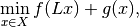
The standard way of fitting this problem into the Chambolle-Pock framework is to summarize both data fit and regularization terms into the composition part $f \circ L$ of the solver, and to set $g$ to the positivity constraint $\iota_{[0, \infty]}$ . By setting $L = (I, \nabla): X \to X \times X^d$ , where $I$ is the identity mapping on $X$ , we can write

$d(x) + r(x) = \left \| \begin{pmatrix} d(x) \\ p(x) \end{pmatrix} \right \|_1 = \left \| \begin{pmatrix} \|x - y\|_2^2 / 2 \\ \lambda \|\nabla x\|_1 \end{pmatrix} \right \|_1 = \big[ f \circ L \big](x)$

with the functional $f: X \times X^d \to \mathbb{R}$ defined by

$f(x, u) = \left \| \begin{pmatrix} \|x - y\|_2^2 / 2 \\ \lambda \|u\|_1 \end{pmatrix} \right \|_1 = \frac{1}{2} \|x - y\|_2^2 + \lambda \|u\|_1.$

Note that the arguments $x, u$ of $f$ are independent, i.e. the sum of the two functionals is a SeparableSum.

Note

The operator $L$ maps $X$ to the ProductSpace $X \times X^d$ . Such a “one-to-many” type of mapping is also called BroadcastOperator.

Numerical solution using ODL¶

Now we implement a numerical solution to the above defined problem using the Chambolle-Pock solver in ODL.

Problem setup¶

The first step in the problem setup is the definition of the spaces in which we want to solve the problem. In this case, we use an $L^2$ space on the square $[0, 100] \times [0, 100]$ . We choose 256 discretization points per axis:

>>> space = odl.uniform_discr(min_pt=[0, 0], max_pt=[100, 100], shape=[256, 256])

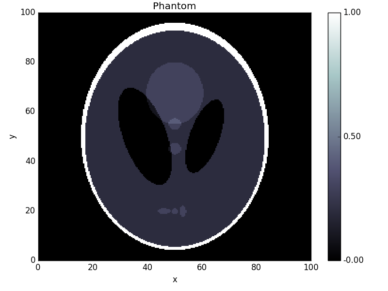
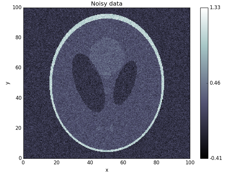
In real problems, the data $y$ would be given by some measurement, but for the purpose of testing the solver, we generate data by creating a modified Shepp-Logan phantom and adding 10% Gaussian noise:

>>> phantom = odl.phantom.shepp_logan(space, modified=True)
>>> data = phantom + odl.phantom.white_noise(space) * 0.1

We now need to define the forward operator $L$ , which we do one constituent at a time:

>>> ident = odl.IdentityOperator(space)
>>> grad = odl.Gradient(space)

To create $L$ , we use the BroadcastOperator class as mentioned above:

>>> L = odl.BroadcastOperator(ident, grad)

We can now proceed to the problem specification. This step requires us to specify the functionals $f$ and $g$ , where the former is the SeparableSum of the squared $L^2$ distance to $y$ and the (vectorial) $L^1$ norm. These functionals are available in ODL as L2NormSquared and L1Norm, respectively:

>>> l2_norm_squared = odl.solvers.L2NormSquared(space).translated(data)
>>> l1_norm = 0.0003 * odl.solvers.L1Norm(grad.range)
>>> f = odl.solvers.SeparableSum(l2_norm_squared, l1_norm)

Note

We don’t need to take extra care of the $L^1$ norm being a vectorial norm since L1Norm also works on product spaces.

Finally, we define the functional for the nonnegativity constraint, available as the functional IndicatorNonnegativity:

>>> g = odl.solvers.IndicatorNonnegativity(space)

Calling the solver¶

Now that the problem is set up, we need to select some optimization parameters. For the Chambolle-Pock method, there is one main rule that we can use: The product of the primal step $\tau$ , the dual step $\sigma$ and the squared operator norm $\|L\|^2$ has to be smaller than 1, $\tau \sigma \|L\|^2 < 1$ . Apart from this, there are no clear rules on how to select $\tau$ and $\sigma$ – basically we’re left with trial and error. We decide to pick them both equal to $1 / \|L\|$ . To calculate an estimate of the operator norm, we have the tool power_method_opnorm which performs the simple power iteration to approximate the largest singular value of $L$ :

>>> op_norm = 1.1 * odl.power_method_opnorm(L, maxiter=4, xstart=phantom)
>>> tau = sigma = 1.0 / op_norm

Finally, we pick a starting point (zero) and run the algorithm:

>>> x = space.zero()
>>> odl.solvers.chambolle_pock_solver(
...     x, f, g, L, tau=tau, sigma=sigma, niter=100)

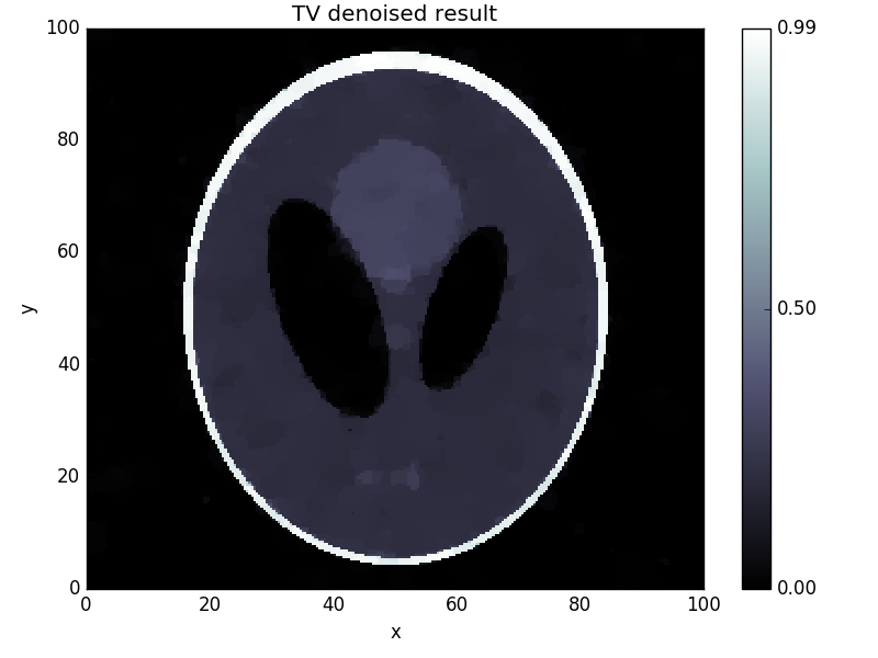
Now we check the result after 100 iterations and compare it to the original:

>>> fig1 = phantom.show('phantom')
>>> fig2 = data.show('noisy data')
>>> fig3 = x.show('TV denoised result')

This yields the following images: